Although ecology doesn’t have many general laws, one most likely to qualify is the species-area relationship. If you walk through a field in a straight line and count all the different species you come across, you’ll notice that the total number of species increases as you progress along your straight path. After a while, however, you’ll start seeing the same species over and over again until you eventually find that you’re no longer spotting any new ones. This is the asymptotic species-area curve. While the exact mathematical form of the relationship is still hotly debated, it is safe to assume that it is an increasing function that reaches a plateau once all the species have been encountered.

An obvious extension of this non-linear relationship is that the numbers of species driven to extinction increases exponentially as larger areas of habitat are destroyed. Species can endure moderate habitat destruction because they can persist in the remaining tracts of land. But as the area being destroyed increases, species are restricted to smaller and smaller patches of habitat until, eventually, they can no longer survive. As a consequence, the extinction of species due to the destruction of the last 10% of a rainforest will be orders of magnitude greater than the number of extinctions caused by destroying the first 10%.

From a human perspective, this suggests that nature can withstand small amounts of interference from our activities. Society depends on natural resources; only the most die-hard tree-hugger would deny this. The challenge is to strike a balance between our destruction and the conservation of species.

One of the greatest advancements in conservation during the 20th century was the Environmental Impact Assessment (EIA), which is now compulsory in most countries across the planet. A simple explanation of the EIA process is that it aims to identify and quantify the positive and negative impacts of any proposed development. This allows decision-makers to formulate informed judgements on whether or not the development is justifiable from the standpoint of sustainable development.

While the world with EIA is undoubtedly better than one without it, the entire process is far from perfect. Most EIAs only focus on a single local development and its potential effect on the immediate surroundings. But, as we’ve already seen, many ecological systems do not respond to stressors in a linear way. The basic EIA process doesn’t handle non-linearities particularly well.

Fortunately, non-linearities can be incorporated into the EIA process through Cumulative Effects Assessments (CEA). CEA understands that although the addition of a second development might double the potential benefit to society, it does not just lead to a twofold increase the negative ecological effects. Instead, the negative impacts scale exponentially because the total effect of the second development is the sum of its local impact and its contribution to the cumulative regional impact.

All this arm-waving can be clarified with a simple example: imagine a project to develop a mine in a pristine ecosystem. The EIA process argues that the project can commence only if the eventual benefits to society (e.g. raw materials, employment, social upliftment) outweigh the negative impacts on the environment (e.g. pollution, habitat destruction, species extinctions).

Let’s assume that permission is granted to the first mine and the miners start digging.

A second mine also wants to join, so it initiates its own EIA as well as a CEA. Theoretically, the second mine should only be granted permission if its eventual benefits outweigh its TOTAL negative impacts. This total is determined as the sum of the local impact (which would be similar to the first mine) and the cumulative impact (which increases exponentially as more and more mines join in).

Astute readers would’ve realised that this is not a very fair system because any developer arriving slightly late will be faced by rapidly increasing cumulative impacts, which were partly caused by its predecessors.

Such a system has two terrible consequences First, developers have massive incentives to beat their competitors in order to avoid responsibility for escalating cumulative impacts. This cultivates a culture of exploitative-urgency, which undermines the tenets of the precautionary principle. Second, developers will be encouraged to exploit untouched, pristine ecosystems where they will not face any cumulative impacts. They will be the first to leave footprints in the sand, so to speak.

________________________________________

This problem has bothered me for the past 3 years. However, because it was not the immediate focus of my PhD research, I relegated it to the back of my mind and devoted my attention to other questions instead.

This changed last year, while I was helping my PhD advisor, Bram Vanschoenwinkel, with his sampling campaign in Western Australia as part of his research. I told him about my troubles with the CEA process during one of the long car drives between survey locations. The distraction-free weeks of sleeping in tents without computers, email and the internet, inspired us to come up with a simple simulation framework to explore my concerns.

Armed with only notebook and pencil, we came up with a caricature of reality that could explain some of the problems with CEA.

---

Step 1: First we needed a landscape of individual patches.

---

Step 2: We then seeded these patches with independent species of different levels of occupancy (Range size).

---

Step 3: The number of species in each patch was used a metric for the local impact, should that specific patch be destroyed. This represented the number of species that would go locally extinct as a consequence of the development of the patch.

---

Step 4: Values representing the local benefit were arbitrarily assigned to the patches, while ensuring that the average local impact was equal to the average local benefit across the entire landscape.

---

Step 5: We used a simple equation to quantify each patch’s contribution to the cumulative impacts based on the number of species in the landscape and their range sizes. This could be interpreted as the number of species that would go extinct in the landscape should that patch be destroyed.

---

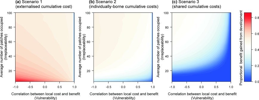
Step 6: We then compared three scenarios to examine how the incorporation of cumulative impacts into the decision-making process influenced the number of patches that were ultimately destroyed and the total benefit that could be accrued from their destruction. These scenarios were:

Externalised cumulative costs: cumulative impacts were completely ignored and decisions were made solely by comparing local impacts (species richness) to the local benefit.

Individually-born cumulative costs: a patch could be destroyed if the local benefit was greater than the total cost (local impact + cumulative impact). Here cumulative costs were carried by individual developers, so latecomers faced larger cumulative costs than the pioneers.

Shared cumulative costs: again, a patch could be destroyed if the local benefit was greater than the total cost (local impact + cumulative impact). This scenario differed in that the total cumulative cost of the entire landscape was first quantified using the equation from step 5 and then divided equally across all the patches regardless of the order of their destruction. In this scenario, all developers faced equal costs for cumulative impacts.

---

Step 7: As a final step, we varied the vulnerability and irreplaceability of the landscape. Vulnerability was manipulated by changing the correlation between local costs and local benefits. A vulnerable patch would be one containing many species while also offering high benefits for development. Irreplaceability represents how much the destruction of any individual patch contributes to the total species extinction across the landscape and was modelled by varying the average range size of species across the landscape.

---

After returning from Australia, I spent a few of days whipping up the above 7 steps into an R script and we wasted little time writing up the results, which have just been published in the Journal for Nature Conservation.

So what did we find? You should read the whole article for the details, but I’ll briefly summarise them here.

• Including cumulative impacts in the decision-making process reduced the number of patches being destroyed as well as the benefit obtained from development.
• Sharing the cumulative costs across all patches (Scenario 3) further decreased the number of patches destroyed and also the benefit obtained from development. In our discussion section we argued that this is probably the most “fair” way to incorporate cumulative impacts into environmental decision-making, but this is open to personal interpretation.
• Lastly, we showed that the differences between these three decision-making strategies were greatest in landscapes with high vulnerability and high irreplaceability.

---

Even though our conclusion were based on a simulation model that has yet to be tested in the real world, the findings were quite disheartening. If our toy model demonstrates anything, it’s that the decisions we make on how to best achieve sustainable outcomes may have the greatest impact in regions of the greatest conservation concern. Our choices have the greatest consequences in instances where the stakes are the highest. I think we should take this responsibility more seriously than we are now.

---

Buschke, F.T. and Vanschoenwinkel, B. 2014. Mechanisms for the inclusion of cumulative impacts in conservation decision-making are sensitive to vulnerability and irreplaceability in a stochastically simulated landscape. Journal of Nature Conservation, 22, 265-271. (If you can’t access the full article, just leave a comment below and I’ll send it to you – copyright rules)