One of the most fruitful sub-fields in ecology is using climate variables to predict species’ geographic distributions. For the uninitiated, species distribution modelling assumes that species are limited in their distributions to suitable climate zones. By studying the environmental conditions where species are known to occur, you can infer the total geographic distribution by calculating the suitability of unsampled regions based on the environmental. Furthermore, using the same principle, species distribution modelling can forecast the effect of future climate change of the distribution of life on earth.

Unfortunately, studies have shown that these fancy climate-based techniques cannot consistently outperform much simpler ones based on spatial phenomena. For instance, spatial interpolation between point occurrences outperforms sophisticated climate-based predictions. Similarly, elaborate climate-based predictions perform no better than expected from random chance.

The trouble lies in the spatially-structured world we live in. Species distributions, especially at large spatial scales, are spatially-autocorrelated due to constrained dispersal. Similarly, climate variables are also spatially structured because the meteorological processes at proximal regions are generally more similar than those at distant sites.

When trying to link species distributions to climate conditions, the challenge lies is separating spatial and environmental correlations in species distributions. Specifically, we should identify three patterns in the geographical species distributions.

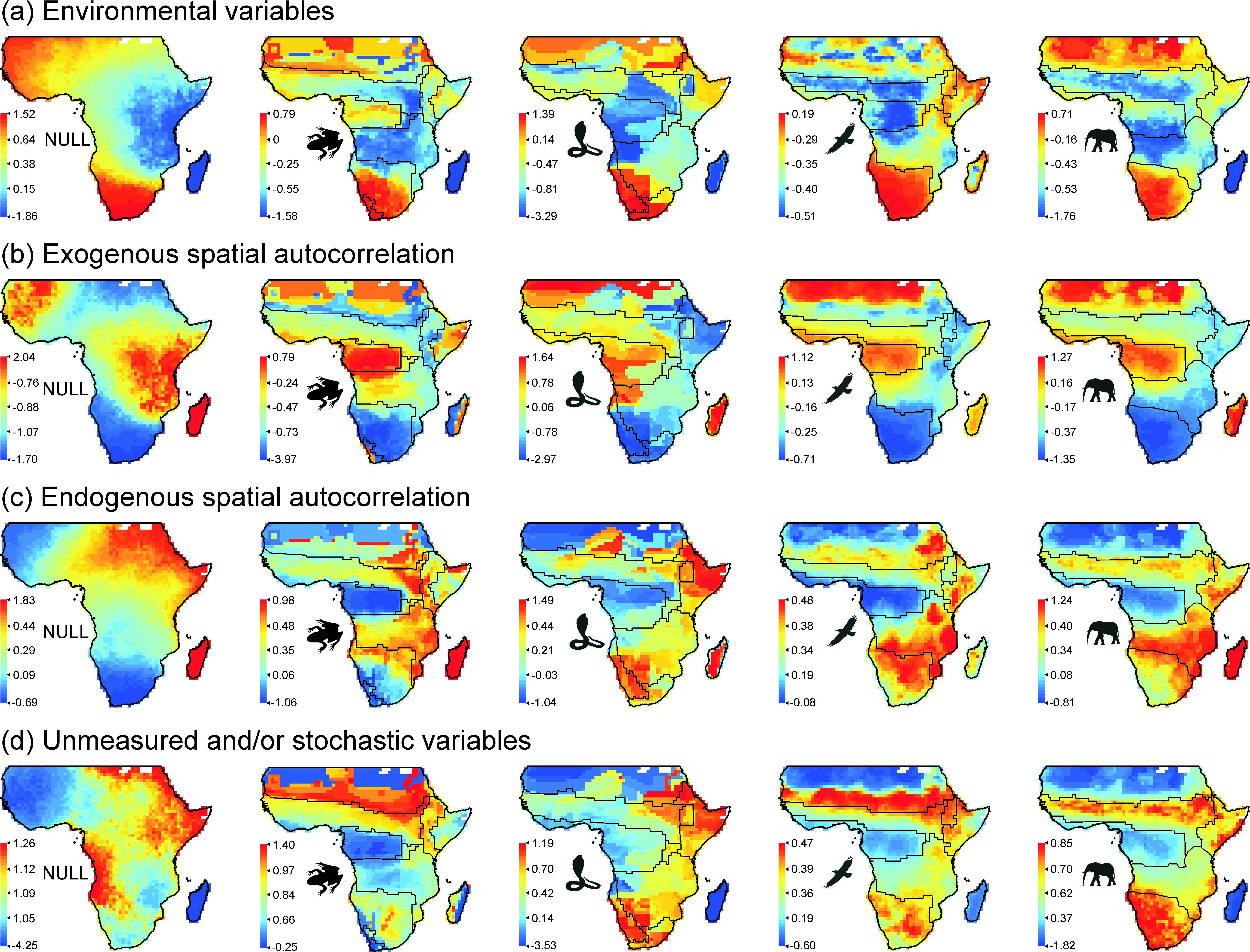
• We must first identify ‘true’ correlations with the environment, which are independent of spatial patterns (E|S).
• Next, we must identify the environmental-associations that also have a strong spatial structure (E∩S). This is known as exogenous spatial autocorrelation because it is due to autocorrelation is the underlying variables.
• Finally, we need to identify spatial patterns that are completely independent of environmental conditions (S|E). This is called endogenous spatial autocorrelation because it supposedly stems from spatial processes, such as dispersal.

In our latest study just published online at Ecography, we set out to quantify the degree of environmental correlation, exogenous and endogenous spatial autocorrelation in the distributions of 4 423 species of amphibians, reptiles, birds and mammals in Africa.

We used variation partitioning to decompose the variation in species ranges into three components of environmental correlation (E|S), exogenous (E∩S) and endogenous spatial autocorrelation (S|E). Variation partitioning assumes that the total variation in a phenomena always sums to 1 (100%). Each of the three components (E|S, E∩S, S|E) are proportions of the total variation. This also allows us to calculate the proportion of unexplained variation using simple arithmetic.

In addition, we also simulated two different null models to test whether patterns for real species are indicative of true underlying ecological mechanisms.

• The first null model (Random Model) scattered simulated species randomly across Africa. Because these simulated species were not constrained by dispersal or environmental conditions, any variation in their ranges would be due to the extent of their distributions.
• The second null model (Spatial Model) was a spreading dye model, which assigned a simulated species to a random starting point and allowed it to expand it range into adjacent areas, regardless of environmental conditions. Any variation is these simulated species would be due to the combined effects of range size and range cohesiveness caused by dispersal limitation.

Our results surprised us. As the extent of a species distribution increases, so does the amount of variation in it range explained by environmental associations (E|S) and exogenous spatial autocorrelation (E∩S). The amount of variation explained by endogenous spatial autocorrelation (S|E) had a hump-shaped relationship with range size. Unexplained variation decreases when species are more widely-distributed.

The Random null model failed to demonstrate any of these patterns, indicating that they are not merely the consequence of range size.

Unfortunately, similar patterns appeared in the Spatial null model. This suggests that the general effect of range size observed in real species is due to range-cohesiveness cause by limited dispersal and not explicit climate-based ecological mechanisms! This raises doubts about the usefulness of climate-based species distribution models because we failed to find evidence for causal relationships between climate and species distributions.

However, not all patterns were spurious. When we looked at the residuals of the relationship between the variation components and species range size, we uncovered something remarkable. Species with more or less prevalent environmental and spatial patterns in their distributions (compared to an average species with the same range size) tended to co-occur. Moreover, these patterns of co-occurrence coincided almost perfectly with the boundaries between biogeographical regions in Africa!

What’s more, these clear biogeographical patterns did not arise in the simulated species.

(Please excuse the bright colours: WordPress insists on using RGB colours instead of CMYK.)

These biogeographical patterns suggest that the importance of environmental associations, exogenous and endogenous spatial autocorrelation depend on geographic locality and the biogeographical region in which species occur. This may indicate that the importance of underlying ecological processes (i.e. dispersal-based vs. niche-based mechanisms) are not universal, but are instead the consequence of the same historical processes that shaped biogeographical patterns in Africa.

Here’s the reference to our paper (feel free to contact me if you cannot gain access):

Buschke, F.T., De Meester, L., Brendonck, L. & Vanschoenwinkel, B. (2014) Partitioning the variation in African vertebrate distributions into environmental and spatial components – exploring the link between ecology and biogeography. Ecography, 37, early view. doi: 10.1111/ecog.00860