Aspiring scientists quickly learn that where they publish their hard earned data is important for career progression. A paper in a prestigious journal pushes them up the professional ladder faster than the same paper in an obscure one.

This has led to an obsession with quantifying the prestige of a journal using impact metrics. Over at Conservation Bytes, Corey Bradshaw presents a RShiny App to rank ecology and conservation journals using a composite of different citation metrics. His app is based on a published paper, so you can be sure that it technically sound. It is not my intention to criticise these efforts; if you want to rank jounals, then this composite approach is definitely the way to go.

However, I don’t think there is much to gain from ranking journals based on their impact metrics. Moreover, scientists – especially early-career scientists – would be better off judging journals based on whether is will ensure that their paper reaches the right audience.

Before anyone thinks I’m naive, I realise that scientists are regularly evaluated for jobs, promotions or grants. In many cases, the people doing the evaluating will just look at journal impact factors or quartile range. I’ve done it myself. I am also not suggesting that all journals are equal. They aren’t. Some are definitely better than others, not only in terms of prestige, but also in terms of readership, editorial policies, historical track-records and contributions to scientific societies. So, scientists should definitely consider where journals fit in the quality hierarchy… and I chose the word hierarchy on purpose.

We shouldn’t see journals as a queue, where the journal at the front of the queue is superior to all those behind it. Instead, we should see journals as branches of a tree, where some branches are more sturdy than others, but twigs on the same branch are equally solid.

This begs the question: how should we distinguish between branches on the journal tree? Its pretty simple really. In fact, Corey Bradshaw showed us how in his original paper (Figure 3). It is possible to cluster journals based on their impact metrics, so that their relationships are a hierarchical tree instead of a ranking (code available at the end of this post). Here is an example for Ecology journal using the same impact metrics used for multidimensional rankings:

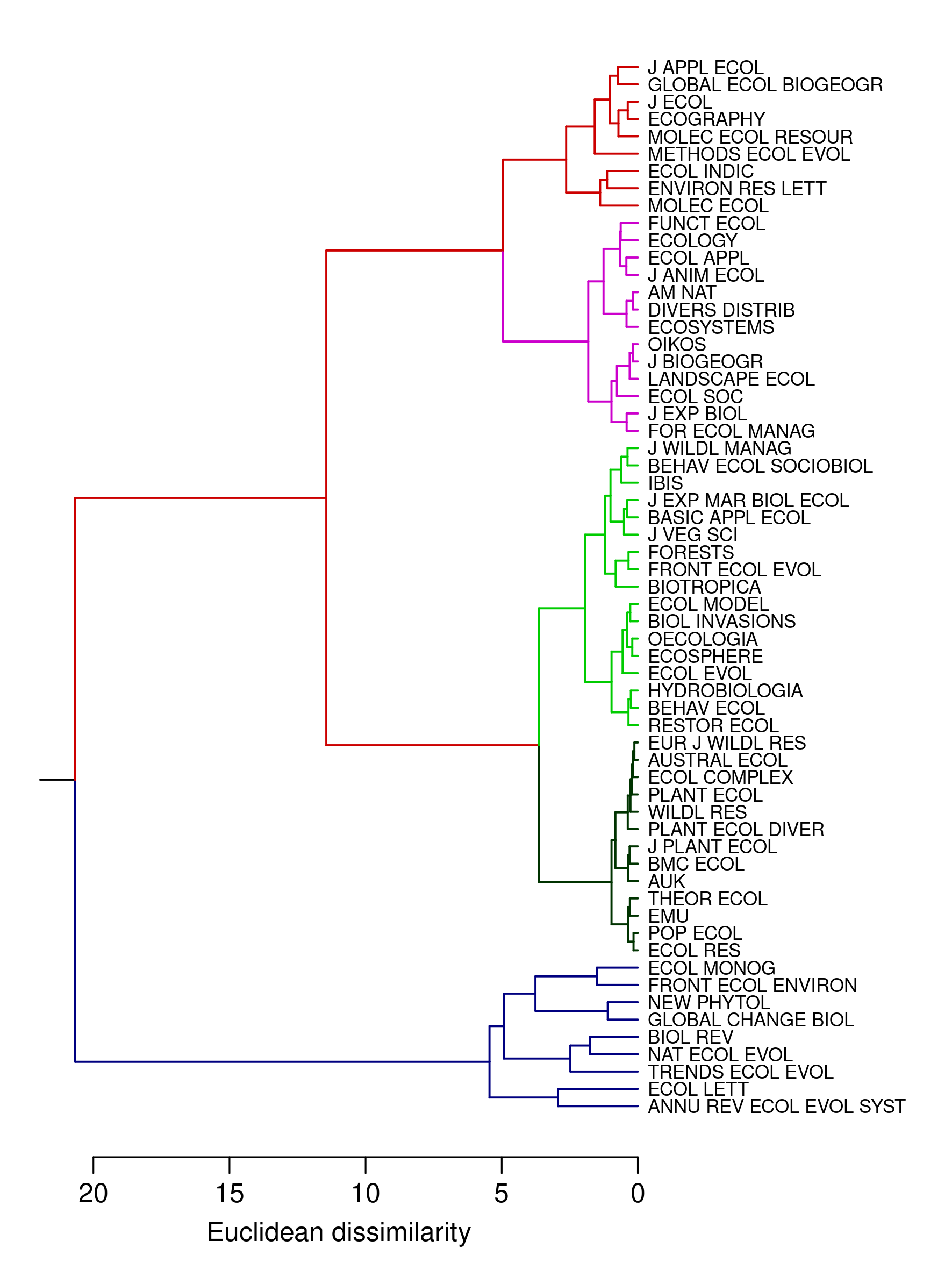
What is immediately obvious is that there are only five clusters, which are much easier to grapple with than the ranking of the 61 journals in this sample. My main argument is that we should only rank journals to the extent of distinguishing between different clusters. Trying to distinguish between journals within clusters based on impact metrics seems pointless to me. Instead, we should rather distinguish between these journals using subjective criteria like scope, readership, or general fit.

For example, the dark blue cluster includes all the journals with the highest impact metrics. In many cases, you can distinguish between these journals based on their scope and whether your paper would fit there. Review papers (e.g. TREE, Biological Reviews), short papers (e.g. Ecology Letters, Nature Ecology and Evolution), longer papers (e.g. Ecological Monographs), or applied papers (e.g. Frontiers in Ecology and the Environment, Global Change Biology) should each be sent to the most appropriate journal. But there are no material career consequences of publishing in one of these journals instead of the others.

Similarly, distinguishing between the red and pink clusters tells you more about the types of papers than the quality of the journals. For example, papers in Methods in Ecology and Evolution will generally be cited more often than papers in American Naturalist, but not necessarily because they make a bigger contribution to the field. Methods papers will be cited more often than primary research simply because they are more likely to be applied across different research sub-disciplines (the same comparison applies to Ecography and Journal of Biogeography, because the former publishes software papers and the latter doesn’t).

So, while scientists should have a general idea of where a journal fits in the hierarchical tree, they needn’t fixate on impact metrics beyond that. Focusing on impact metrics can lead to an flood of submissions to journals even when there is no realistic chance of being accepted due to lack of fit. This wastes scientists’ and editors’ time and demoralises early-career researchers who get rejected from one journal to the next without peer-review. Science as a whole would be better off if we all submitted our research to journals where it is most likely to reach the right readership. Often, this won’t be the journal with the most impressive impact metrics.

# Open  dataset
Jdata <- read.csv("Jsamp2019.csv", na.strings = "NULL")
# Download from: https://github.com/cjabradshaw/JournalRankShiny/blob/main/Jsamp2019.csv

# The cluster analysis requires the 'vegan' package in R. 
# First install the package and then load it to the session
#install.packages("vegan")
library(vegan)

clust.dat <- scale(Jdata[,4:9])

rownames(clust.dat) <- Jdata[,1]

######################################################################
######################################################################

# Save Figure 2 in the working directory as a PNG File

png(filename="Cluster.png",width=15,height=20,units="cm",res=300)

# This clusters the data and saves it as a dendrogram based on:
  # - Euclidean distance,
  # - Ward's amalgamation rule
clust <- as.dendrogram(hclust(vegdist(clust.dat,"euclidean"), "ward.D2"))

# The following function identifes nodes in the cluster dendrogram
# and assigns each its own colour.
colbranches <- function(n, col)  {
  a <- attributes(n) # Find the attributes of current node
  # Color edges with requested color
  attr(n, "edgePar") <- c(a$edgePar, list(col=col, lwd=1.25))
  n # Don't forget to return the node!
  }

# Create an cluster object (called 'clust2') and define it as a dendrogram
clust2 <- as.dendrogram(as.hclust(clust), hang = 0.35)

# Color the first branch in blue,
clust2[[1]] = dendrapply(clust2[[1]], colbranches, rgb(0,0,0.5,1))
# Color the other branches in shades of green and red,
clust2[[2]][[1]][[1]] = dendrapply(clust2[[2]][[1]][[1]], colbranches, rgb(0,0.2,0,1))
clust2[[2]][[1]][[2]] = dendrapply(clust2[[2]][[1]][[2]], colbranches, rgb(0,0.8,0,1))
clust2[[2]][[2]][[1]] = dendrapply(clust2[[2]][[2]][[1]], colbranches, rgb(0.8,0,0.8,1))
clust2[[2]][[2]][[2]] = dendrapply(clust2[[2]][[2]][[2]], colbranches, rgb(0.8,0,0,1))
clust2[[2]] = dendrapply(clust2[[2]], colbranches, rgb(0.8,0,0,1))

# Set margins for plot
par(mai=c(0.7,0.1,0.1,1.8))
# This plots the cluster dendrogram
plot(clust2, center=F,las=1, xlab="Euclidean dissimilarity",horiz=T, edgePar = list(col = 2:3),
     nodePar = list(lab.cex = 0.7, pch = NA), mgp=c(1.8,0.6,0),
      edge.root =T, main = "")

dev.off() # Close plot device and save file